Summary

This project developed a real-time distance measurement system using two Sharp GP2Y0A02YK infrared range sensors to detect an approaching object over a 0 cm to 150 cm measurement range. The target requirement was at least 10% accuracy, and the final system achieved less than 2% mean percentage error through sensor calibration, analog filtering, digital filtering, moving-average smoothing, and region-based sensor fusion. The project combined experimental calibration, Arduino-based data acquisition, signal processing, and audio feedback into a complete sensing system.

The system used a staggered two-sensor arrangement to overcome the limited close-range performance of a single IR sensor. Sensor 1 measured the longer range, while Sensor 2 was placed 25 cm behind Sensor 1 to cover the near-field region. The raw analog sensor readings were mapped to physical distance using a nonlinear reciprocal calibration model. To reduce noise, each signal passed through an RC low-pass filter, a third-order Butterworth digital filter implemented using a Biquad structure, and a six-sample moving average. The final distance estimate was also mapped to an audio frequency using an Arduino speaker output.

1. Sensor Calibration

The Sharp GP2Y0A02YK sensors used in this experiment produce analog ADC values that vary nonlinearly with distance due to their internal optical triangulation mechanism. Therefore, the raw ADC values from the Arduino cannot be directly interpreted as physical distance, and a calibrated mapping is required.

To perform the calibration, distance measurements were taken at 5 cm intervals from 20 cm to 150 cm using a standardized setup with a white planar target placed perpendicular to the sensor axis. Calibration data was collected under real-time operational conditions, with both sensors active and filtering applied. To capture the effect of noise, multiple measurements were recorded at each distance.

The following reciprocal model was used for calibration:

In this model, R is the estimated distance in centimeters, V is the measured sensor ADC value, and A, B, and C are calibration constants determined through nonlinear least-squares regression. The regression process adjusted the constants to minimize the error between measured distances and model-predicted distances. This reciprocal model produced good distance-estimation accuracy over the reliable sensor range, approximately 20 cm to 125 cm, with mean percentage error below 2%.

2. Staggering Sensors

Two IR sensors (Sharp GP2Y0A02YK, range 20 to 150 cm) were staggered as demonstrated in Figure-1 at a height of 4cm from the ground. Sensor-1 was located at the zero (starting) position of the obstacle to measure distances from 20 cm to 150 cm. To enable our system measure from 0 to 20 cm that Sensor-1 is unable to measure, we positioned Sensor-2 at a 25cm distance behind Sensor-1 along the direction of measurement/object movement. A distance of 13cm was set widthwise to minimize interference between the two sensors.

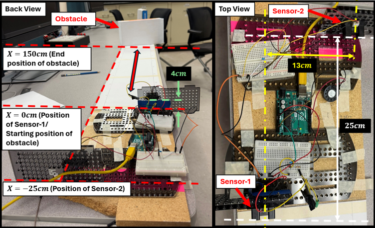
Figure-1: Setup for staggering two IR sensors for measuring 0 to 150cm distance

3. Filtering

Significant noise from the environment and sensor crosstalk affected the signals, so an analog filter, a digital filter, and a moving average were applied to reduce noise while limiting delay. Each sensor signal first passed through an RC low-pass filter (4.7 kΩ, 1 μF; 34 Hz cutoff), then was sampled at 100 Hz and processed by a 3rd-order Butterworth digital low-pass filter with a 1 Hz cutoff. To further reduce the Gaussian noise at the Butterworth output, a moving average was applied: the filtered signal was sampled every 0.21 s (4.76 Hz), converted to distance, averaged over a 6-sample window, and displayed as the final measurement.

Two main challenges arose: minimizing delay and implementing the digital filter on the Arduino. The moving average introduced the most delay. This was mitigated by increasing its sampling rate and reducing its window size. Additionally, the standard difference-equation implementation of the digital filter failed due to Arduino floating-point precision limits (6–7 significant digits). This was resolved by using a Biquad implementation (Arm 2022; Deneberg, et al., 2004) of the second-order section and gain coefficients computed using MATLAB’s butter and zp2sos functions.

4. Sensor Fusion

Since each sensor’s measurement error was substantially below 10%, a region-based fusing strategy was adopted. Sensor-1 (the sensor in front) can only measure from 20 cm to 150 cm, Sensor-2 needed to measure 0 cm to (at least) 20 cm. However, the 20 cm mark was not a good switching point since Sensor-1 had a significant amount of noise at that position. Therefore, a conditional logic was set to enable Sensor-2 to measure distance until 30 cm, and Sensor-1 to measure from 30 cm to 150 cm.

5. Mapping Distance Measurements to Notes

The final system used a speaker to play a sound based on the measured distance. The distance measurement was normalized over the range from 0 cm to 165 cm, where 165 cm represents 10% beyond the required 150 cm maximum range. The normalized value was then mapped to a frequency between 200 Hz and 2000 Hz and played using Arduino’s tone() function.

6. Conclusion

This project demonstrated a complete dual-IR-sensor distance measurement system capable of measuring object distance from 0 cm to 150 cm with accuracy well above the required threshold. The system combined nonlinear calibration, physical sensor staggering, analog filtering, digital Butterworth filtering, moving-average smoothing, region-based sensor fusion, and audio feedback. The project highlighted the importance of stable sensor mounting, careful calibration, hardware-aware filter implementation, and system-level design in achieving robust real-time sensing performance.

References

• ARM. (2022). Biquad Cascade IIR Filters Using Direct Form I Structure. CMSIS DSP Software Library.
• Denenberg, J., et al. (2004). Filter Design.

Appendix A – Arduino Code

The Arduino code below implements IR sensor sampling, Biquad-based Butterworth filtering, reciprocal distance calibration, region-based sensor fusion, moving-average smoothing, serial output, and speaker-based tone feedback.

/* PIN DEFINITIONS */
int IRpin1 = A1;
int IRpin2 = A2;
int speakerOut = 9;

/* TONE MAPPING PARAMETERS */
#define FREQ_MIN 200
#define FREQ_MAX 2000

const float DISTANCE_MIN = 0.0;
const float DISTANCE_MAX = 165.0;

/* MOVING AVERAGE SETUP */
#define MA_WINDOW 6
float buffer[MA_WINDOW] = {0};
float sum = 0;
int index = 0;

/* SENSOR CALIBRATION */
const float sensor2_offset = 25.0;

// Sensor 1 calibration model coefficients
const float A_1 = 1.23072369e+04;
const float B_1 = 1.12642133e+01;
const float C_1 = 1.74338869e+00;

// Sensor 2 calibration model coefficients: 25 cm to 55 cm fit
const float A_2 = 2.26723367e+04;
const float B_2 = 9.58009427e+01;
const float C_2 = -1.29063311e+01;

/* SAMPLING PARAMETERS */
const unsigned long sampleTime = 10000;       // microseconds
const unsigned long outputSampleTime = 210000; // microseconds

unsigned long prevTime = 0;
unsigned long prevOutputTime = 0;

float filtered_ADC_sensor_1;
float filtered_ADC_sensor_2;

/* DIGITAL FILTER BIQUAD STRUCT DEFINITIONS */
struct Biquad {
  float b0, b1, b2;
  float a1, a2;
  float x1, x2;
  float y1, y2;
};

struct ButterworthFilter {
  Biquad s1;
  Biquad s2;
};

struct BiquadCoeff {
  float b0, b1, b2;
  float a1, a2;
};

struct BiquadState {
  float z1, z2;
};

struct ButterworthState {
  BiquadState sensor1State;
  BiquadState sensor2State;
};

/* DIGITAL FILTER INITIALIZATION */
const BiquadCoeff stage1Coeff = {
  2.91464944656977e-05f,
  2.91464944656977e-05f,
  0.0f,
  -0.939062505817492f,
  0.0f
};

const BiquadCoeff stage2Coeff = {
  1.0f,
  2.0f,
  1.0f,
  -1.93529438685999f,
  0.939120798806424f
};

ButterworthState filterIR1 = {0};
ButterworthState filterIR2 = {0};

/* ALL LOGIC IMPLEMENTED BELOW */
float processBiquad(const BiquadCoeff &c, BiquadState &s, float x) {
  float y = c.b0 * x + s.z1;
  s.z1 = c.b1 * x - c.a1 * y + s.z2;
  s.z2 = c.b2 * x - c.a2 * y;
  return y;
}

float processButterworth(ButterworthState &f, float x) {
  float y = processBiquad(stage1Coeff, f.sensor1State, x);
  y = processBiquad(stage2Coeff, f.sensor2State, y);
  return y;
}

float getDistance(float filtered_ADC_sensor_1, float filtered_ADC_sensor_2) {
  float R1 = A_1 / (filtered_ADC_sensor_1 + B_1) + C_1;
  float R2 = (A_2 / (filtered_ADC_sensor_2 + B_2) + C_2) - sensor2_offset;

  // Use Sensor 2 when the distance is below 30 cm
  if (R2 < 30) {
    if (R2 < 0.9) {
      return 0.0;
    }
    return R2;
  }

  return R1;
}

float movingAverage(float x) {
  sum -= buffer[index];
  buffer[index] = x;
  sum += x;

  index++;
  if (index >= MA_WINDOW) {
    index = 0;
  }

  return sum / MA_WINDOW;
}

void setup() {
  pinMode(speakerOut, OUTPUT);
  Serial.begin(115200);
  prevTime = micros();
  prevOutputTime = micros();
}

void loop() {
  unsigned long currTime = micros();

  // Sample only after sampleTime has passed
  if (currTime - prevTime >= sampleTime) {
    float ADC_sensor1 = analogRead(IRpin1);
    float ADC_sensor2 = analogRead(IRpin2);

    filtered_ADC_sensor_1 = processButterworth(filterIR1, ADC_sensor1);
    filtered_ADC_sensor_2 = processButterworth(filterIR2, ADC_sensor2);

    prevTime += sampleTime;
  }

  // Compute distance and play sound only after outputSampleTime has passed
  if (currTime - prevOutputTime >= outputSampleTime) {
    float R = getDistance(filtered_ADC_sensor_1, filtered_ADC_sensor_2);
    R = movingAverage(R);

    Serial.println(R);

    float normalized = (R - DISTANCE_MIN) / (DISTANCE_MAX - DISTANCE_MIN);
    int frequency = FREQ_MIN + normalized * (FREQ_MAX - FREQ_MIN);

    tone(speakerOut, frequency);

    prevOutputTime += outputSampleTime;
  }
}

Appendix B – Calibration Code in Python

The Python code below fits the reciprocal calibration model using calibration data from Excel files and evaluates the mean absolute and percentage errors.

import pandas as pd
import numpy as np
from scipy.optimize import curve_fit

# Convert calibration data into the required long format
def melt_sensor_adc(path):
    df = pd.read_excel(path).drop(columns=["Distance(cm)"])
    long = df.melt(var_name="distance_cm", value_name="adc").dropna()
    long["distance_cm"] = long["distance_cm"].astype(float)
    long["adc"] = long["adc"].astype(float)
    return long


def restrict_range(df, lo=20, hi=150):
    return df[(df["distance_cm"] >= lo) & (df["distance_cm"] <= hi)].copy()


def drop_outliers_iqr(df):
    cleaned = []

    for d, g in df.groupby("distance_cm"):
        q1, q3 = g["adc"].quantile([0.25, 0.75])
        iqr = q3 - q1
        lo, hi = q1 - 1.5 * iqr, q3 + 1.5 * iqr
        cleaned.append(g[(g["adc"] >= lo) & (g["adc"] <= hi)])

    return pd.concat(cleaned, ignore_index=True)


# Reciprocal calibration model using ADC as the independent variable
def model_adc(V, A, B, C):
    return A / (V + B) + C


def fit_model_adc(train_df):
    train_mean = train_df.groupby("distance_cm", as_index=False)["adc"].mean()

    V = train_mean["adc"].values
    R = train_mean["distance_cm"].values

    A0 = (R.max() - R.min()) * V.mean()
    B0 = 10.0
    C0 = R.min() - 5

    bounds = ([0.0, 0.001, -200.0], [1e6, 500.0, 200.0])

    popt, _ = curve_fit(
        model_adc,
        V,
        R,
        p0=[A0, B0, C0],
        bounds=bounds,
        maxfev=500000
    )

    return popt


def evaluate_adc(df, popt):
    pred = model_adc(df["adc"].values, *popt)
    true = df["distance_cm"].values

    abs_err = np.mean(np.abs(pred - true))
    eps = 1e-6
    pct_err = np.mean(np.abs(pred - true) / np.maximum(true, eps)) * 100

    return abs_err, pct_err


# ---------------- Sensor 1 ----------------
s1 = drop_outliers_iqr(
    restrict_range(melt_sensor_adc("Sensor1.xlsx"), 20, 150)
)

# ---------------- Sensor 2 ----------------
s2 = drop_outliers_iqr(
    restrict_range(melt_sensor_adc("Sensor2.xlsx"), 20, 150)
)

# 70/30 split by distance bins
distances = np.array(sorted(s1["distance_cm"].unique()))
test_dist = set(distances[::3])
train_dist = set(distances) - test_dist

train_df = s1[s1["distance_cm"].isin(train_dist)].copy()
test_df = s1[s1["distance_cm"].isin(test_dist)].copy()

print(f"Train distances: {len(train_dist)} Test distances: {len(test_dist)}")

p1_adc = fit_model_adc(train_df)
train_abs, train_pct = evaluate_adc(train_df, p1_adc)
test_abs, test_pct = evaluate_adc(test_df, p1_adc)

print("Sensor 1 fitted on ADC (A, B, C):", p1_adc)
print(f"TRAIN: mean abs err = {train_abs:.2f} cm, mean % err = {train_pct:.2f}%")
print(f"TEST : mean abs err = {test_abs:.2f} cm, mean % err = {test_pct:.2f}%")


def sensor1_distance_from_adc(adc):
    A, B, C = 1.23072369e+04, 1.12642133e+01, 1.74338869e+00
    return A / (adc + B) + C


print(sensor1_distance_from_adc(75))

Appendix C – MATLAB Code

The MATLAB code below computes the third-order Butterworth filter coefficients and converts them to second-order sections for Biquad implementation on Arduino.

Fs = 100;
fc = 1;
order = 3;

Wn = fc / (Fs / 2);

[z, p, k] = butter(order, Wn, 'low');
[sos, g] = zp2sos(z, p, k)