
Projects
Visual Servoing System for Object Tracking
Summary
This project focused on the design, implementation, and analysis of a vision-based servo tracking system with an objective of understanding how feedback control can be applied to track a moving object using image-based measurements in a mechatronic system. Through this project, multiple system components, including image processing, communication, and control, were integrated to achieve real-time tracking performance. The experiment demonstrated how system dynamics such as delay and phase lag affect tracking accuracy, particularly at higher input frequencies. It also highlighted the importance of controller tuning and the limitations imposed by sensing and actuation in practical systems.
1. System Overview and Working Principles
The objective of this project was to develop a visual servoing system capable of tracking a green tennis ball and maintaining it at the center of the camera’s field of view. Fig. 1 demonstrates the setup that consisted of a USB camera and a green tennis ball, each mounted on separate 180° rotation servo motors fixed to a table surface. The camera was connected to a Raspberry Pi 5, which performed all image acquisition and processing using Python and the OpenCV library. The servo motors were controlled by an Arduino Uno, with serial communication established between the Raspberry Pi and Arduino.
The system operated as a closed-loop feedback system. The camera continuously captured images, detected the tennis ball, and computed the ball center position in pixel coordinates. This information was transmitted to the Arduino, which adjusted the camera servo angle to reduce the horizontal offset between the ball’s position and the image center. This process repeated in real time, with the system minimizing tracking error through continuous feedback.
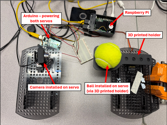 Figure 1: Set-up for visual servoing system.
2. Tennis Ball Detection Algorithm
The computer vision task in this experiment was to detect the presence of a tennis ball in an image and estimate its center coordinates. This was achieved using a color-based segmentation approach.
First, the image was converted into a suitable color space (HSV), and lower and upper bounds corresponding to the green color of the tennis ball were defined. The cv2.inRange() function was then applied to generate a binary mask, where pixels within the specified color range were set to white and all others to black. Erosion and dilation, in that order, were used to remove small noise and undesired features such as the curved line pattern on the tennis ball, while preserving the overall shape of the object.
Next, cv2.findContours() was used to extract the contours from the processed binary image. The detected contours were sorted based on their area, and the largest contour was selected under the assumption that only one ball is present in the scene. Finally, cv2.minEnclosingCircle() was applied to the largest contour to fit a circle around it. The center and radius of this circle were used as an estimate of the tennis ball’s position and size in pixel coordinates.
3. Control System Design
The control objective was to actuate the camera servo such that the ball remains at the center of the image frame. Since only horizontal motion was considered, the problem was formulated as a regulation problem with the image center as the reference. The control input was the commanded camera servo angle, while the ball motion was considered a disturbance or external input.
A discrete-time proportional-derivative (PD) controller was used for tracking. Let xball,i be the horizontal position of the ball in the image at time step i, and xcenter the constant image frame center. The tracking error was defined as:
Let ui denote the commanded camera servo angle at time step i. The control law is given by:
where Kp and Kd are the proportional and derivative gains, respectively. The term (ei − ei−1) is used to approximate the time derivative of the error by absorbing the sampling interval into Kd. The controller was tuned at 1 Hz ball frequency. Starting from zero, Kp was increased until oscillatory behavior was observed, after which Kd was increased to attenuate the oscillations without significantly slowing the system response. The final gain values used were Kp = 0.08 and Kd = 0.15.
4. Other Software Implementation Details
The algorithms described in the preceding sections were implemented on a Raspberry Pi in Python and an Arduino. Certain considerations about the system required that some features be added in implementing this system. They are discussed below.
4.1. Ball Motion Generation
The ball motion was generated by commanding the servo with a sinusoidal input at a user-specified frequency. The servo was centered at 90°, with an initial commanded amplitude of 75°. However, as the input frequency increased, the observed motion amplitude decreased. This is attributed to the limited dynamic response of the servo to increasing ball inertia, which was unable to track rapid command changes. As a result, the servo exhibits low-pass behavior.
This effect introduced an error in the logged data, since the actual servo angle was not directly measured and was instead approximated by the commanded input. At higher frequencies, this assumption becomes inaccurate due to the reduction in actual amplitude. To address this, the commanded amplitude was adjusted as a function of frequency to remain within the achievable range of the servo. The relationship was determined empirically by observing the maximum achievable amplitude across frequencies. The final expression used was:
4.2. Communication and Data Logging
Since camera servo actuation depends on ball detection, the Raspberry Pi and Arduino communicate over a serial connection. Serial communication was initialized at a baud rate of 9600 on both the Raspberry Pi and Arduino. The horizontal pixel coordinate of the detected ball center is filtered using a moving average over a window of five samples to reduce measurement noise. The filtered value is encoded as a single byte and transmitted to the Arduino.
In addition to transmitting position data, the Raspberry Pi issues control commands to manage data logging. Upon receiving a logging command, the Arduino records timestamped ball and camera servo angles during operation. Due to memory constraints, the number of stored samples was limited to 300 per trial. When commanded by the Raspberry Pi, the Arduino transmits the stored data back to the Raspberry Pi, where it is saved as a CSV file for subsequent analysis. A simple byte-based protocol is used to distinguish between data and control signals: values in the range 0–249 represent valid ball center positions, 254 indicates a command to start logging, and 255 indicates a command to stop logging and return the stored data.
5. Testing and Analysis
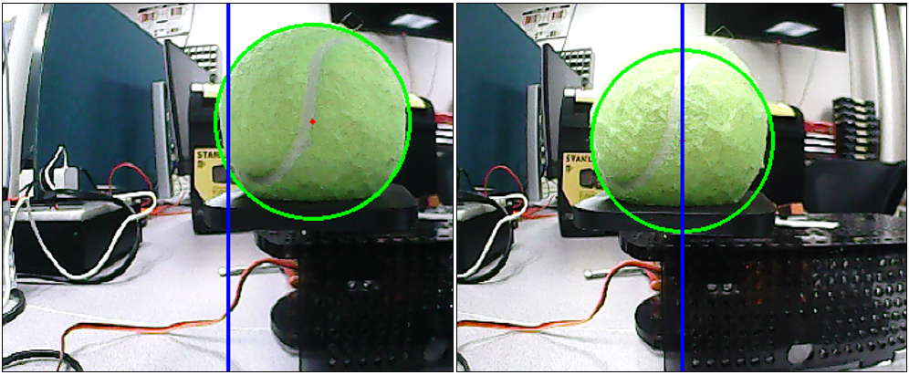
The full code implementations of the visual servoing system are in Appendix A. The system was tested by commanding the ball servo at different frequencies ranging from 0.4 Hz to 2.0 Hz. The camera was able to track the ball such that the full ball shape was always in the frame. Fig. 2 shows frame captures from the camera during operation. However, as frequency increased, the camera lagged more behind the ball. The ball servo also exhibited increased jitter at lower frequencies. At these frequencies, the controller commands small angular changes that fall below the servo’s 1° resolution. These commands accumulate and are executed as sudden larger movements, resulting in visible jitter.
At each frequency, data was collected as described in Section 4.2. A sinusoidal wave was fitted to the camera servo data at each frequency. The amplitude and phase of each wave was compared to the ball motion to determine gain and phase difference. These values were then plotted as Bode magnitude and phase plots to analyze system behavior across frequencies as shown in Fig. 3.
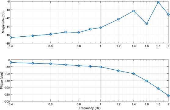 Figure 3: Magnitude and phase response of the system as a function of input frequency.
The magnitude plot shows that the system attenuates the input signal, with gain remaining below 0 dB across all frequencies. The phase plot shows that the phase lag increases with frequency. At low frequencies, the phase lag is relatively small, indicating good synchronization between the input and output. However, as frequency increases, the phase lag becomes much larger, showing that the system response is increasingly delayed. Overall, the system behaves like a low-pass system, performing well at lower frequencies but struggling to track higher-frequency inputs accurately.
The transport delay was estimated by directly measuring the time taken by the Python vision pipeline, from image acquisition and processing to sending the control signal to the Arduino. The data in Table 1 shows that the delay remains nearly constant across all tested frequencies, with an average value of approximately 0.0337 seconds. Minor variations are observed due to computational and communication fluctuations, but overall, the delay is largely independent of frequency, which is consistent with the definition of transport delay.
| Frequency (Hz) | Code running time (s) |
|---|---|
| 0.4 | 0.0426760310001554 |
| 0.8 | 0.0313555278330568 |
| 1.2 | 0.028947963499983114 |
| 1.6 | 0.034521631166323154 |
| 2.0 | 0.031092906833085483 |
6. Conclusion
This project implementated a visual servoing system in which a Raspberry Pi-based vision algorithm detected the horizontal position of a tennis ball and commanded a camera servo via an Arduino using a discrete-time PD controller. Observations demonstrated that visual servoing systems are strongly affected by sensing delay, actuator limitations, and processing speed. While the controller performed well at low frequencies, the increasing phase lag at higher frequencies highlighted the importance of system dynamics and real-time constraints. The experiment also demonstrated how image-based measurements can be effectively used for feedback control, but are sensitive to noise and detection accuracy. One remaining question is how the system performance would improve with more advanced control strategies, such as full PID control or model-based approaches. Additionally, it will be interesting to investigate whether incorporating direct measurement of the servo angle could reduce tracking error.
References
- OpenCV, “Contour Features,” OpenCV Documentation, 2018.
- K. J. Åström and R. M. Murray, Feedback Systems: An Introduction for Scientists and Engineers. Princeton, NJ, USA: Princeton University Press, 2021, ch. 11.
- Arduino, “Arduino Uno Rev3,” Arduino Documentation.
Appendix A – Code Implementation
A.1. Raspberry Pi Python Code
import numpy as np
import cv2
import serial
import time
from datetime import datetime

CMD_BALL_LOST = 253
CMD_START_LOGGING = 254
CMD_DUMP_LOG = 255

cap = cv2.VideoCapture(0, cv2.CAP_V4L2)
cap.set(cv2.CAP_PROP_FRAME_WIDTH, 480)
cap.set(cv2.CAP_PROP_FRAME_HEIGHT, 360)

ser = serial.Serial('/dev/ttyACM0', 9600, timeout=0.2)
time.sleep(2)
ser.reset_input_buffer()
ser.reset_output_buffer()

lower_tennis = np.array([25, 50, 50])
upper_tennis = np.array([60, 255, 255])

x_history = []
window_size = 5
transport_delay = [0,0,0,0,0,0]
delay_i = 0

timestamp_str = datetime.now().strftime("%Y%m%d_%H%M%S")
save_filename = f"servo_log_{timestamp_str}.csv"

while True:
    start_time = time.perf_counter()
    grabbed, frame = cap.read()
    if not grabbed:
        print("Failed to grab frame")
        break

    frame_width = frame.shape[1]
    frame_height = frame.shape[0]
    frame_center_x = frame_width // 2

    hsv = cv2.cvtColor(frame, cv2.COLOR_BGR2HSV)
    threshold_hsv = cv2.inRange(hsv, lower_tennis, upper_tennis)
    threshold_hsv = cv2.erode(threshold_hsv, None, iterations=2)
    threshold_hsv = cv2.dilate(threshold_hsv, None, iterations=2)

    contours, _ = cv2.findContours(threshold_hsv, cv2.RETR_TREE, cv2.CHAIN_APPROX_SIMPLE)

    if len(contours) > 0:
        largest_contour = max(contours, key=cv2.contourArea)
        (x, y), radius = cv2.minEnclosingCircle(largest_contour)
        center = (int(x), int(y))

        if radius > 10:
            cv2.circle(frame, center, int(radius), (0, 255, 0), 2)
            cv2.circle(frame, center, 2, (0, 0, 255), -1)

            x_history.append(x)
            if len(x_history) > window_size:
                x_history.pop(0)
            x_filtered = sum(x_history) / len(x_history)

            x_byte = int((x_filtered / (frame_width - 1)) * 249)
            x_byte = max(0, min(249, x_byte))
            ser.write(bytes([x_byte]))
            print(f"x raw = {x:.1f}, x filtered = {x_filtered:.1f}, sent = {x_byte}")
        else:
            x_history.clear()
            ser.write(bytes([CMD_BALL_LOST]))
            print("Ball too small, sent = 255 (return servo to center)")
    else:
        x_history.clear()
        ser.write(bytes([CMD_BALL_LOST]))
        print("Ball not found, sent = 255 (return servo to center)")

    end_time = time.perf_counter()
    transport_delay[delay_i] = end_time - start_time
    delay_i = (delay_i + 1) % len(transport_delay)

    cv2.line(frame, (frame_center_x, 0), (frame_center_x, frame_height), (255, 0, 0), 2)
    cv2.imshow('HSV Image', threshold_hsv)
    cv2.imshow('frame', frame)

    key = cv2.waitKey(1) & 0xFF
    if key == 27 or key == ord('q'):
        print("\nExit key pressed. Requesting Arduino log dump...")
        break
    elif key == 27 or key == ord('w'):
        print("Telling Arduino to start logging")
        ser.write(bytes([CMD_START_LOGGING]))

cap.release()
cv2.destroyAllWindows()

ser.reset_input_buffer()
ser.write(bytes([CMD_DUMP_LOG]))
ser.flush()
time.sleep(0.5)

lines = []
log_started = False
start_time = time.time()
timeout_seconds = 10

while True:
    if time.time() - start_time > timeout_seconds:
        print("Timed out while waiting for Arduino log data.")
        break
    raw = ser.readline()
    if not raw:
        continue
    line = raw.decode('utf-8', errors='ignore').strip()
    if not line:
        continue
    print("RX:", line)
    if line == "LOG_BEGIN":
        log_started = True
        lines = []
        continue
    if line == "LOG_END":
        print("Finished receiving log data.")
        break
    if log_started:
        lines.append(line)

if lines:
    with open(save_filename, "w") as f:
        for line in lines:
            f.write(line + "\n")
    print(f"Saved Arduino log to: {save_filename}")
else:
    print("No log data received, so no file was saved.")

print("Transport delay: " + str(sum(transport_delay)/len(transport_delay)))
ser.close()
A.2. Arduino Code
#include <Servo.h>
#include <math.h>

Servo camServo;
Servo ballServo;

const int camServoPin = 12;
const int ballServoPin = 11;

const uint8_t CMD_START_LOGGING = 254;
const uint8_t CMD_DUMP_LOG = 255;

float camCurrentAngle = 90.0;
const float camCenterAngle = 90.0;
const float Kp = 0.08;
const float Kd = 0.15;
float prevError = 0.0;
const float camServoMin = 20.0;
const float camServoMax = 160.0;
const int centerByte = 125;

const float frequency = 0.4;
const float ballCenterAngle = 90.0;
float ballAngle = ballCenterAngle;
float amplitude = 30.0 * (0.3 - frequency) + 75.0;

unsigned long lastCamUpdate = 0;
const unsigned long camUpdateInterval = 20;
unsigned long lastBallUpdate = 0;
const unsigned long ballUpdateInterval = 20;

const int MAX_SAMPLES = 300;
uint16_t logTime[MAX_SAMPLES];
uint8_t logCamAngle[MAX_SAMPLES];
uint8_t logBallAngle[MAX_SAMPLES];
int logCount = 0;

const unsigned long logInterval = 50;
unsigned long lastLogTime = 0;
unsigned long testStartTime = 0;
bool logRequested = false;
bool dumpRequested = false;

int angleToMicroseconds(float angleDeg) {
    if (angleDeg < 0.0) angleDeg = 0.0;
    if (angleDeg > 180.0) angleDeg = 180.0;
    return (int)(1000.0 + (angleDeg / 180.0) * 1000.0);
}

void logSampleIfNeeded(unsigned long now) {
    if (logCount >= MAX_SAMPLES) return;
    if (now - lastLogTime >= logInterval) {
        lastLogTime = now;
        unsigned long elapsed = now - testStartTime;
        logTime[logCount] = (uint16_t)elapsed;
        logCamAngle[logCount] = (uint8_t)round(camCurrentAngle);
        logBallAngle[logCount] = (uint8_t)round(ballAngle);
        logCount++;
    }
}

void dumpLogToSerial() {
    Serial.println("LOG_BEGIN");
    Serial.println("timestamp_ms,cam_angle_deg,ball_angle_deg");
    for (int i = 0; i < logCount; i++) {
        Serial.print(logTime[i]);
        Serial.print(",");
        Serial.print(logCamAngle[i]);
        Serial.print(",");
        Serial.println(logBallAngle[i]);
    }
    Serial.println("LOG_END");
}

void handleSerialByte(int xByte) {
    if (xByte == CMD_START_LOGGING) {
        logRequested = true;
        testStartTime = millis();
        return;
    }
    if (xByte == CMD_DUMP_LOG) {
        dumpRequested = true;
        return;
    }
    if (xByte >= 0 && xByte <= 249) {
        float error = xByte - centerByte;
        float derivative = error - prevError;
        float controlOutput = Kp * error + Kd * derivative;
        camCurrentAngle += controlOutput;
        if (camCurrentAngle > camServoMax) camCurrentAngle = camServoMax;
        if (camCurrentAngle < camServoMin) camCurrentAngle = camServoMin;
        camServo.write((int)round(camCurrentAngle));
        prevError = error;
    }
}

void setup() {
    Serial.begin(9600);
    camServo.attach(camServoPin);
    ballServo.attach(ballServoPin);
    camServo.write((int)round(camCurrentAngle));
    ballServo.writeMicroseconds(angleToMicroseconds(ballCenterAngle));
    lastLogTime = millis();
}

void loop() {
    unsigned long now = millis();

    if (dumpRequested) {
        camServo.write((int)round(camCurrentAngle));
        ballServo.writeMicroseconds(angleToMicroseconds(ballAngle));
        dumpLogToSerial();
        while (true) {
            delay(1000);
        }
    }

    if (now - lastBallUpdate >= ballUpdateInterval) {
        lastBallUpdate = now;
        float t = (now - testStartTime) / 1000.0;
        ballAngle = ballCenterAngle + amplitude * sin(2.0 * PI * frequency * t);
        if (ballAngle > 180.0) ballAngle = 180.0;
        if (ballAngle < 0.0) ballAngle = 0.0;
        ballServo.writeMicroseconds(angleToMicroseconds(ballAngle));
    }

    if (now - lastCamUpdate >= camUpdateInterval) {
        lastCamUpdate = now;
        while (Serial.available() > 0) {
            int xByte = Serial.read();
            handleSerialByte(xByte);
        }
    }

    if (logRequested) {
        logSampleIfNeeded(now);
    }
}
A.3. Data Analysis Code
clc; clear; close all;

%% ===== LOAD FILES =====
folder_name = 'Final logger lab5';
files_struct = dir(folder_name);
files = {files_struct.name};
files = files(3:end); % remove . and ..

freqs_input = [0.4:0.1:1.0, 1.2:0.2:2]';

assert(length(files) == length(freqs_input), ...
    'Mismatch between files and frequencies');

%% ===== PREALLOCATE =====
gains = zeros(length(files),1);
phases = zeros(length(files),1);

%% ===== MAIN LOOP =====
for k = 1:length(files)
    filename = files{k};
    f = freqs_input(k);
    disp(['Processing: ', filename]);

    data = readmatrix([folder_name,'/',filename]);

    t = data(:,1) / 1000;
    cam = data(:,2);
    ball = data(:,3);

    cam = cam - mean(cam);
    ball = ball - mean(ball);

    start_idx = round(0.3 * length(t));
    t = t(start_idx:end);
    cam = cam(start_idx:end);
    ball = ball(start_idx:end);

    w = 2*pi*f;
    X = [sin(w*t), cos(w*t)];

    theta_cam = X \ cam;
    a = theta_cam(1); b = theta_cam(2);
    A_cam = sqrt(a^2 + b^2);
    phi_cam = atan2(b, a);

    theta_ball = X \ ball;
    ab = theta_ball(1); bb = theta_ball(2);
    A_ball = sqrt(ab^2 + bb^2);
    phi_ball = atan2(bb, ab);

    gains(k) = A_cam / A_ball;
    phases(k) = phi_cam - phi_ball;

    T = 1/f;
    mask = t <= (t(1) + 2*T);
    t_plot = t(mask);
    cam_plot = cam(mask);
    ball_plot = ball(mask);

    cam_fit_plot = A_cam * sin(w*t_plot + phi_cam);
    ball_fit_plot = A_ball * sin(w*t_plot + phi_ball);

    figure;
    subplot(2,1,1);
    plot(t_plot, cam_plot, 'b', 'LineWidth', 1); hold on;
    plot(t_plot, cam_fit_plot, 'r--', 'LineWidth', 1.5);
    grid on;
    title(['Camera Fit | f = ', num2str(f), ' Hz']);
    legend('Measured', 'Fit');
    ylabel('Camera');

    subplot(2,1,2);
    plot(t_plot, ball_plot, 'b', 'LineWidth', 1); hold on;
    plot(t_plot, ball_fit_plot, 'r--', 'LineWidth', 1.5);
    grid on;
    title(['Ball Fit | f = ', num2str(f), ' Hz']);
    legend('Measured', 'Fit');
    ylabel('Ball');
    xlabel('Time (s)');
end

phases = unwrap(phases);

%% ===== BODE PLOT =====
figure;
subplot(2,1,1);
semilogx(freqs_input, 20*log10(gains), '-o', 'LineWidth', 1.5);
grid on;
ylabel('Magnitude (dB)');

subplot(2,1,2);
semilogx(freqs_input, rad2deg(phases), '-o', 'LineWidth', 1.5);
grid on;
ylabel('Phase (deg)');
xlabel('Frequency (Hz)');