
Projects
Convex Optimization-Based Identification of Linear Dynamical Systems Using Regularization
Convex Optimization-Based Identification of Linear Dynamical Systems Using Regularization
Abstract
System identification is a fundamental problem in robotics and control, where the objective is to estimate unknown system parameters from measured input-output data. This paper presents a convex optimization-based framework for identifying the parameters of a discrete-time linear dynamical system using ordinary least squares and regularized least squares formulations. A second-order single-input single-output linear time-invariant model is considered, where the current output depends on previous output values and current and previous input values. The parameter estimation problem is formulated as an unconstrained convex quadratic optimization problem, and convexity and optimality properties are analyzed using standard results from convex optimization theory. Numerical simulations are performed using synthetically generated noisy training data and a separate test dataset for performance evaluation. The results show that ordinary least squares becomes increasingly sensitive to noise and limited data, producing unstable parameter estimates and poor prediction accuracy. In contrast, regularized least squares improves robustness by shrinking parameter magnitudes and significantly reducing test prediction error. Although the regularized estimates are biased, they provide substantially better generalization performance. The study demonstrates how convex optimization provides an effective framework for system identification under noisy and data-limited conditions.
Index Terms—convex optimization, least squares, regularization, system identification, discrete-time systems
I. Introduction
System identification is a well-established field concerned with estimating mathematical models of dynamical systems from measured input-output data [1]–[3]. Classical approaches include least-squares estimation, prediction-error methods, and maximum-likelihood-based methods [1], which are commonly used for identifying linear dynamical systems when the model structure is known or can be selected from data. These methods provide a strong theoretical foundation and are widely discussed in standard system identification texts. When the system is linear in the unknown parameters, the data can be arranged into a regression form: Aθ ≈ b, and the parameters can be estimated using ordinary least squares. In this setting, ordinary least squares provides a natural and widely used method for estimating the unknown parameter vector. Classical system identification texts describe least-squares estimation as a fundamental approach for identifying linear models from measured data [1]. However, practical identification problems often involve short, noisy, or limited datasets, which can make ordinary least-squares estimates sensitive to measurement noise and lead to poor generalization [4]–[6].
This sensitivity is related to the conditioning of the regression matrix. When the columns of the regression matrix are nearly linearly dependent, the least-squares problem becomes ill-conditioned, so small measurement errors can produce large changes in the estimated parameters [7]–[9]. In system identification, a related issue occurs when the input data do not sufficiently excite the system dynamics, making it difficult to estimate the parameters reliably [1], [2], [10]. As a result, the least-squares solution may fit the available noisy data but fail to represent the true system parameters accurately. This issue becomes more important when the model contains many parameters relative to the number of available data points.
Regularization methods are useful tools for reducing the effect of noise, model uncertainty, and ill-conditioning in least-squares-based estimation problems. A common example is ℓ2-regularization, also known as ridge or Tikhonov regularization. In this method, the squared Euclidean norm of the parameter vector is added as a penalty term. This discourages excessively large parameter values and improves the conditioning of the estimation problem [11]-[13]. Therefore, ℓ2-regularized least squares is especially useful when the regression matrix is ill-conditioned or when the available data are noisy and limited.
Other regularization methods can also be used depending on the desired model behavior. For example, ℓ1-regularization is often used when a sparse parameter vector is desired, because it can push some parameter estimates exactly to zero [14]. In contrast, ℓ2-regularization, also known as ridge or Tikhonov regularization, usually shrinks all parameter values smoothly without necessarily setting them to zero [11]–[13]. Nuclear-norm regularization is another convex approach that is commonly used when a low-rank model structure is desired [15], [16].
In modern system identification, regularization has been developed further through kernel-based and Bayesian approaches. Chen et al. emphasized that model estimation and structure detection using short data records are important challenges in modern system identification [17]. A useful method for model estimation with short datasets is the kernel-based regularization method, which was introduced in [4] and later further studied in [5], [6]. The performance of this method depends on kernel structure design and several studies have been carried out to estimate the underlying parameters, often called the hyper-parameters [18], [19]. However, studies carried out to embed the regularization in the Bayesian framework demonstrated the most effective result [18], [20], leading KRM to outperform ML/PEM equipped with classical model structure. Chen et al. proposed a sparse multiple kernel-based regularization method that combines several fixed kernels and estimates their weights through marginal likelihood maximization [17]. Their approach allows the identification method to capture more complicated system dynamics than single-kernel methods and also promotes sparsity for structure detection.
In addition to least-squares and regularized estimation methods, other important branches of system identification have also been developed. Prediction-error and maximum-likelihood methods provide a general statistical framework for estimating dynamic models, while experiment-design and identification-for-control studies focus on collecting informative data for reliable model estimation and controller design [21]–[26]. Subspace identification methods provide another major class of techniques, especially for estimating state-space models from input-output data. These methods are useful for multivariable systems and avoid some of the nonlinear optimization difficulties that can appear in classical prediction-error approaches [27]–[30].
More recent work has also expanded system identification toward sparse and machine-learning-based approaches. Sparse identification methods aim to discover compact governing equations or dynamic models from data by selecting only the most important terms from a larger library of candidate functions [34]–[36]. Nonlinear black-box modeling and neural-network-based approaches have also been studied for cases where the system dynamics are difficult to represent using simple linear models [37], [38]. Recent physics-informed and neural-network-based methods further show how prior physical knowledge and flexible function approximators can be combined for modeling complex dynamical systems [39], [40].
Compared with these advanced identification methods, the present work focuses on a simpler least-squares-based formulation for a discrete-time linear dynamical system. The purpose is not to develop a new system identification algorithm, but to demonstrate how convex optimization ideas can be used to improve parameter estimation in a clear and computationally simple setting. Ordinary least squares is first used as a baseline estimator, and ℓ2-regularized least squares is then introduced to reduce sensitivity to noisy and limited data. By comparing parameter estimates, training error, test error, and prediction performance, the study shows how regularization improves robustness and generalization even when it introduces bias into the estimated parameters.
II. System Model and Problem Formulation
A linear difference equation that maps the input u(t) to the output y(t) for a single-input single-output, linear time-invariant, causal system, commonly referred to as an equation-error model, can be expressed as in [1]:
Here, the parameters ai and bi are assumed constant over time, implying a linear time-invariant system. The disturbance term e(t) is assumed to be zero-mean white noise.
For a second-order system with n = 2 and m = 2, the model reduces to
Solving for y(t) gives
Assuming a deterministic noise-free system, e(t) = 0, which simplifies (3) to
To express the model in discrete-time dynamical system form, introduce the index shift t = k + 1, such that y(t) = vk+1, y(t − 1) = vk, y(t − 2) = vk−1, u(t − 1) = uk, and u(t − 2) = uk−1. Substituting these into (4), and defining α1 = −a1, α2 = −a2, β1 = b1, and β2 = b2, gives
Here, vk is the system output, uk is the control input, and α1, α2, β1, and β2 are unknown system parameters to be estimated.
A. Least Squares Formulation
Rewriting the model from (5),
where
Collecting N data points gives
where A is the regression matrix formed from past outputs and inputs, and b is the vector of measured future outputs.
The least squares problem is formulated as
which is a standard least squares problem [41].
B. Regularized Least Squares
To improve robustness, a regularization term is introduced:
where λ is a regularization parameter [41].
III. Convexity Analysis
The objective function is
This function is convex because the squared Euclidean norm is convex, the composition of a convex function with an affine mapping preserves convexity, and a nonnegative weighted sum of convex functions is convex. Therefore, the optimization problem is convex, and any local optimum is also a global optimum [41].
IV. Optimality Conditions
For the unconstrained problem, the optimal solution satisfies
Expanding the gradient gives
Setting this expression equal to zero gives
and therefore
This is the normal equation for regularized least squares [41]. For λ > 0, ATA + λI is positive definite, so the regularized problem has a unique solution, even if ATA is singular or poorly conditioned.
V. KKT Conditions
For constrained convex problems, the Karush–Kuhn–Tucker conditions consist of stationarity, primal feasibility, dual feasibility, and complementary slackness [41]. Since the problem considered here is unconstrained, the KKT conditions reduce to the stationarity condition
VI. Numerical Simulation
Although (5) is derived under a deterministic assumption, in practice measurements are noisy. To reflect this, the simulated system output includes an additive noise term:
where εk represents zero-mean Gaussian noise. The identification problem then consists of estimating the parameters of the deterministic model from noisy observations, which naturally leads to a least squares formulation.
The parameters were chosen synthetically to satisfy a stable discrete-time response, with
representing a moderately damped system with input influence distributed over multiple time steps. No claim is made that these values correspond to a specific physical system; they serve as a representative test case for evaluating the identification methods.
The control input was generated as a first-order autoregressive process, where the input noise is independent and identically distributed white Gaussian noise. The autoregressive structure produces a stationary, correlated input signal that provides sufficient excitation for identifying the system parameters [2]. The specific coefficients were chosen to yield a bounded, moderately correlated signal with unit-scale variance appropriate for the system dynamics.
Two datasets were generated to evaluate the performance of the estimation methods. The training dataset consists of a short sequence of samples with relatively high noise, creating a challenging identification problem where overfitting may occur. A separate test dataset without added noise was generated to assess predictive performance.
The training dataset consisted of Ntrain = 12 samples, while the test dataset consisted of Ntest = 60 samples. The training output included additive Gaussian noise with standard deviation 0.35, while the test dataset was generated without measurement noise. The regularization parameter was varied over the interval [10−4, 102] using logarithmically spaced samples.
The parameter vector was estimated using least squares and regularized least squares formulations. The least squares problem is
whereas the regularized least squares problem is
The regularization parameter was selected by minimizing the test mean squared error:
In this simulation, the test dataset is used as a proxy for validation due to the limited amount of data available. In practice, a separate validation set or cross-validation should be used to select the regularization parameter, while the test set should be reserved strictly for final performance evaluation.
VII. Results and Discussion
Fig. 1 shows the noisy training input-output data used for parameter estimation. The short training dataset length, Ntrain = 12, combined with additive noise creates a challenging identification problem, increasing the likelihood of overfitting in the least squares estimation.
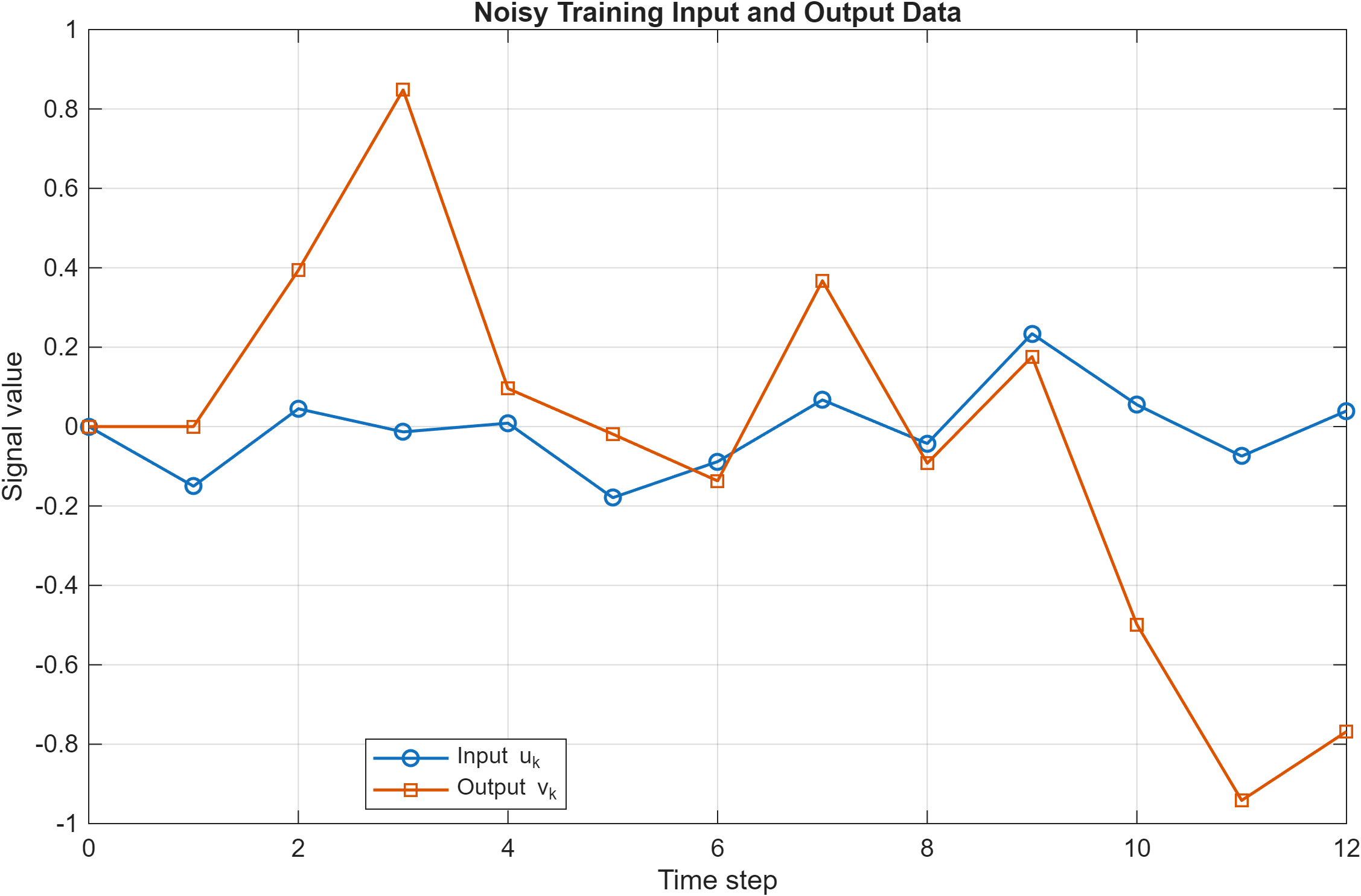
Fig. 1. Noisy training input and output data used for parameter estimation. The short training dataset length, Ntrain = 12, combined with additive measurement noise creates a challenging identification problem and increases the risk of overfitting in the least squares estimate.
The estimated parameters obtained using ordinary least squares and regularized least squares are summarized in Table I and illustrated in Fig. 2. The least squares solution exhibits significant deviation from the true parameters, particularly in the input-related coefficients β1 and β2, where both incorrect signs and large magnitudes are observed. This behavior indicates that the least squares model is highly sensitive to noise and limited training data.
In contrast, the regularized least squares solution produces parameter estimates with substantially smaller magnitudes and reduced overall parameter error. Although the regularized estimates remain biased relative to the true parameters, they are significantly more stable. The parameter estimation error was reduced from 3.5843 for ordinary least squares to 0.8109 for the regularized solution.
| Parameter | True Value | Least Squares | Regularized LS |
|---|---|---|---|
| α1 | 0.6000 | 0.4623 | 0.2695 |
| α2 | -0.2000 | 0.1222 | 0.0381 |
| β1 | 0.5000 | -1.6702 | -0.0632 |
| β2 | 0.3000 | -2.5310 | -0.1177 |
| Parameter Error ‖θ̂ − θtrue‖2 | – | 3.5843 | 0.8109 |
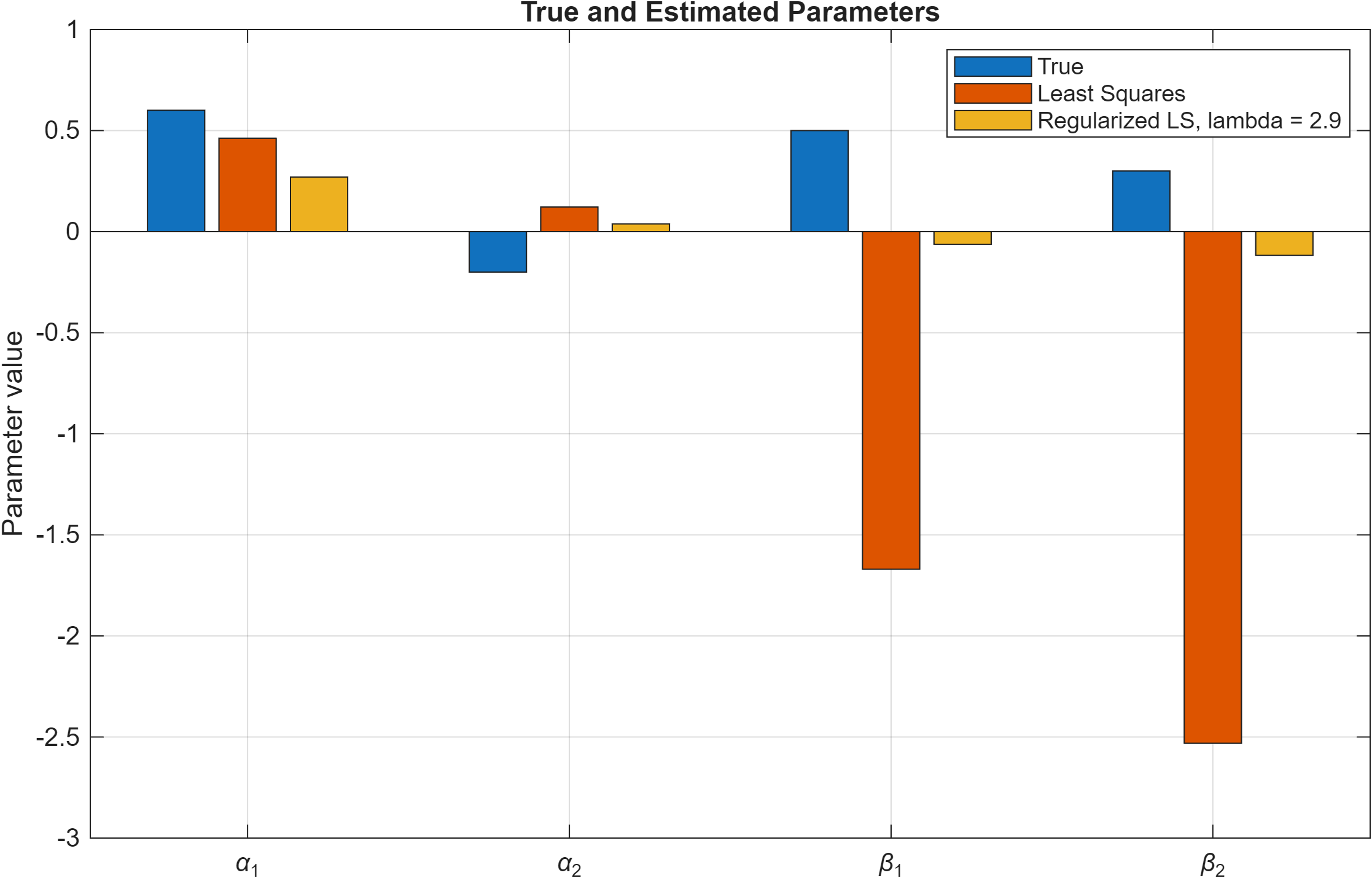
Fig. 2. Comparison of true parameters and estimated parameters obtained using ordinary least squares and regularized least squares. The least squares estimate deviates significantly from the true parameters, especially for the input coefficients β1 and β2, whereas regularization reduces the parameter magnitudes and gives a more stable estimate.
Fig. 3 illustrates the effect of the regularization parameter λ on the estimated parameters. For small values of λ, the regularized solution approaches the ordinary least squares estimate. As λ increases, all parameter estimates progressively shrink toward zero due to the ℓ2-penalty term. This behavior demonstrates how regularization controls model complexity by penalizing large parameter magnitudes.
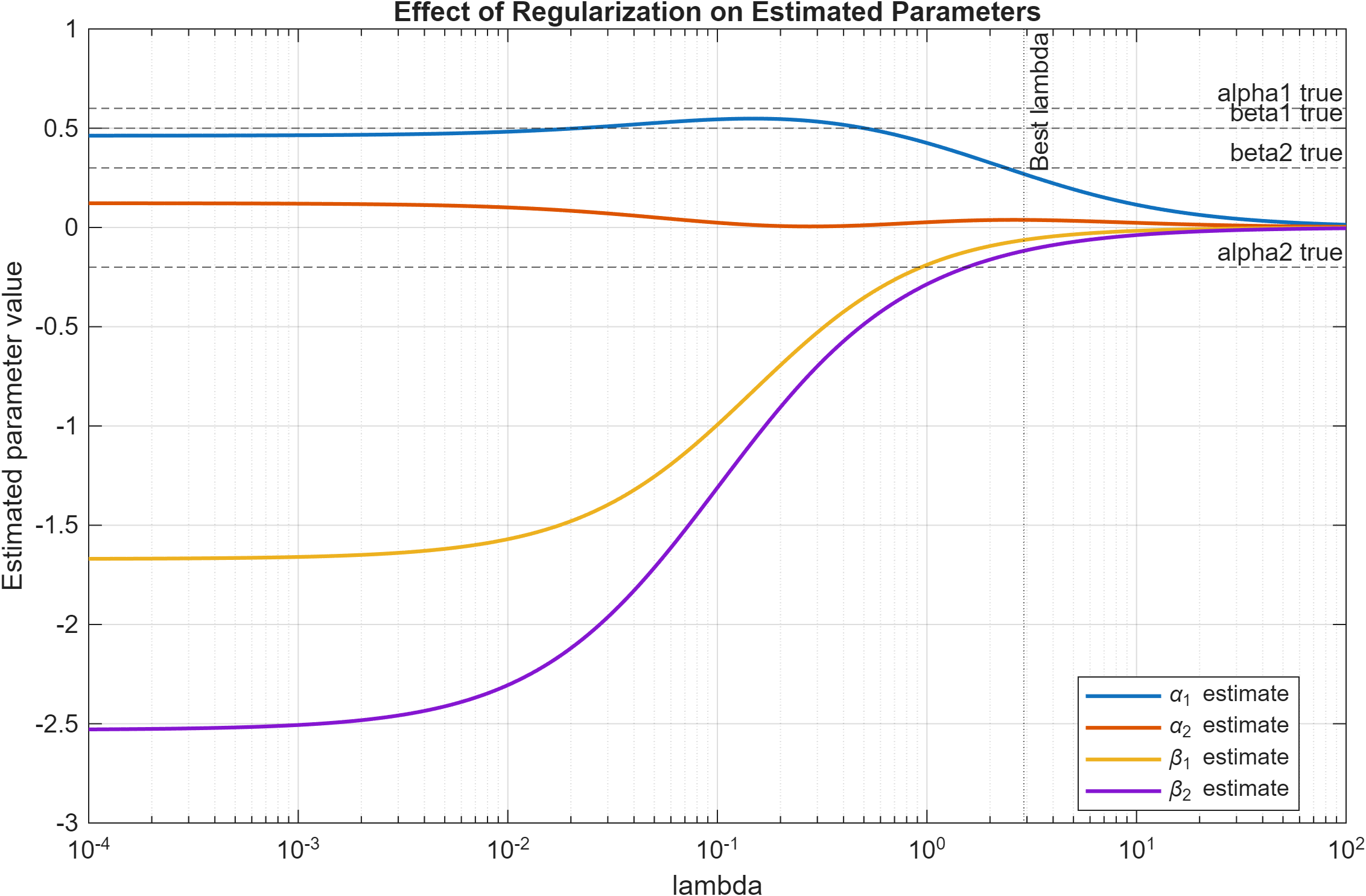
Fig. 3. Effect of the regularization parameter λ on the estimated parameters. For small λ, the solution approaches the ordinary least squares estimate, while increasing λ progressively shrinks the parameters toward zero. The dashed lines indicate the true parameter values, and the vertical line marks the selected value of λ based on minimum test error.
The relationship between regularization and prediction performance is shown in Fig. 4. The training mean squared error increases monotonically with increasing λ, since stronger regularization constrains the model and reduces its ability to fit the training data exactly. In contrast, the test mean squared error initially decreases as overfitting is reduced, reaches a minimum near the selected value of λ, and then increases again for large λ due to underfitting. This behavior clearly demonstrates the classical bias-variance tradeoff associated with regularization.
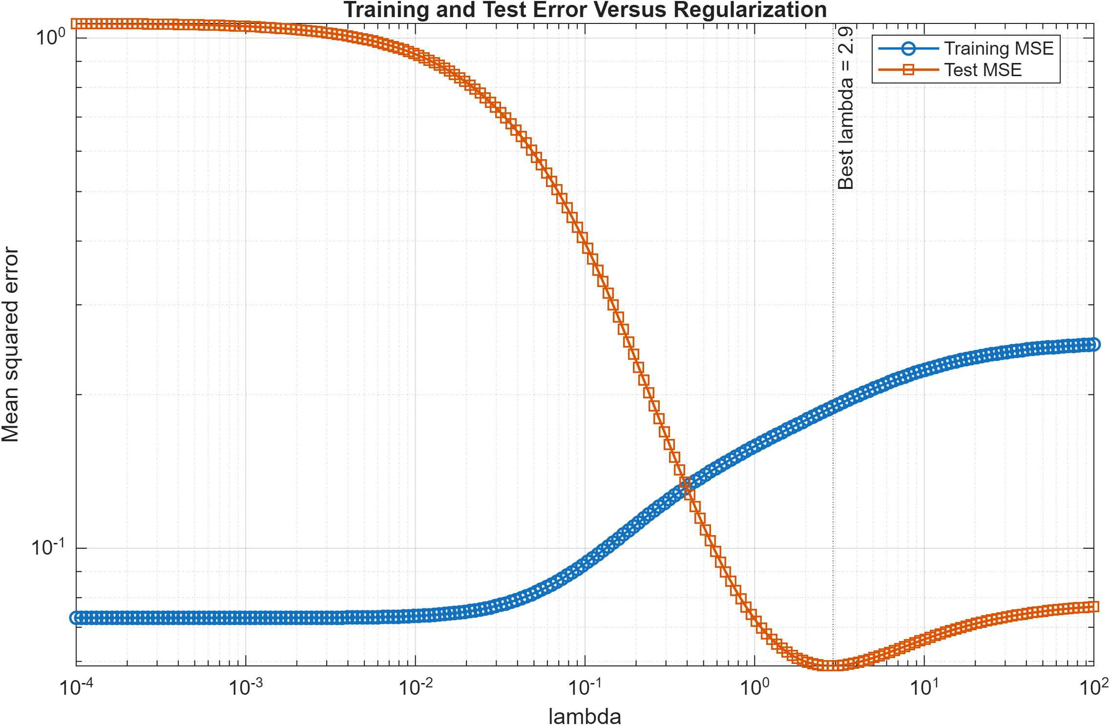
Fig. 4. Training and test mean squared error as functions of the regularization parameter λ. The training error increases monotonically with λ, while the test error reaches a minimum at an intermediate value, illustrating the bias-variance tradeoff and the role of regularization in improving generalization performance.
The predictive performance of the two models is further summarized in Table II. The regularized least squares model reduced the test mean squared error from 1.0696 to 0.0588, corresponding to approximately a 94.5% reduction in prediction error relative to ordinary least squares. This substantial improvement indicates that regularization significantly improves generalization performance under noisy and data-limited conditions.
| Metric | Least Squares | Regularized LS |
|---|---|---|
| Test MSE | 1.0696 | 0.0588 |
| Relative Reduction in Test MSE | – | 94.5% |
The numerical results also highlight the sensitivity of ordinary least squares estimation to limited noisy data. The condition number of the matrix ATtrainAtrain was computed as 31.8852. Although this value does not indicate severe ill-conditioning, it suggests moderate sensitivity of the least squares solution to perturbations in the data. Since the training dataset is both short and noisy, small variations in the measurements can produce large variations in the estimated parameters.
This sensitivity is reflected in Table I, where the least squares estimates for the parameters β1 and β2 exhibit incorrect signs and excessively large magnitudes. Regularization mitigates this effect by modifying the normal equations through the addition of the λI term, which improves numerical stability and reduces sensitivity to measurement noise. As a result, the regularized least squares solution produces substantially improved predictive performance and more stable parameter estimates.
The results also demonstrate the classical bias-variance tradeoff associated with regularization. The ordinary least squares solution corresponds to a low-bias but high-variance estimator, allowing the model to fit the noisy training data aggressively. This leads to unstable parameter estimates and poor predictive performance on unseen data. Increasing the regularization parameter λ introduces bias by shrinking the parameter estimates toward zero. However, this simultaneously reduces variance by decreasing sensitivity to noise and preventing excessively large parameter values. This tradeoff is clearly observed in Fig. 4. For small values of λ, the model overfits the noisy training data, resulting in low training error but high test error. As λ increases, the test error decreases due to improved generalization. Beyond the optimal value of λ, excessive regularization causes underfitting, increasing both training and test errors.
Finally, Fig. 5 compares the predicted outputs on the test dataset. The ordinary least squares model produces highly unstable and high-variance predictions, reflecting severe overfitting to the noisy training data. In contrast, the regularized model produces substantially smoother predictions that more closely follow the overall trend of the true system response.
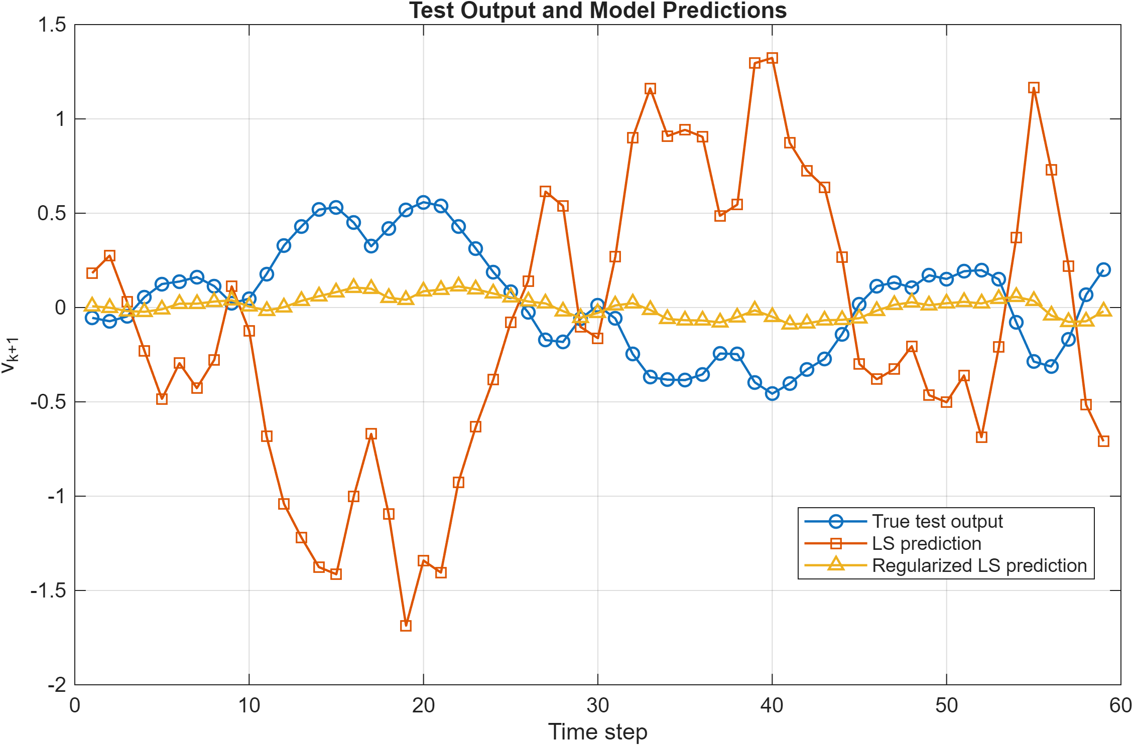
Fig. 5. Comparison of true system output and model predictions on the test dataset. The ordinary least squares model produces high-variance predictions due to overfitting, whereas the regularized least squares model more closely follows the true output trend and demonstrates improved generalization despite biased parameter estimates.
Although the regularized estimates do not recover the true parameters exactly, the results demonstrate that regularization improves predictive performance and robustness by reducing sensitivity to noise and limiting model complexity. Overall, the study highlights the importance of regularization when identifying higher-dimensional dynamical systems from limited noisy data.
VIII. Conclusion
This paper presented a convex optimization-based approach for identifying the parameters of a discrete-time linear dynamical system using ordinary least squares and regularized least squares formulations. A second-order single-input single-output model with four unknown parameters was considered to test the sensitivity of the estimation problem to noise and limited data. The numerical results demonstrated that ordinary least squares can become prone to overfitting under noisy and limited-data conditions, resulting in unstable parameter estimates and poor predictive performance. In contrast, regularized least squares improved robustness by penalizing large parameter magnitudes and substantially reducing test prediction error. Although the regularized estimates were biased, they produced relatively better generalization performance. Overall, the study illustrates how convex optimization provides a reliable and computationally efficient framework for system identification under noisy and data-limited conditions.
Appendix A – MATLAB Code
The MATLAB code used to generate the numerical simulation results is included below for reproducibility.
clear; clc; close all;

%% True system parameters
alpha1_true = 0.60;
alpha2_true = -0.20;
beta1_true = 0.50;
beta2_true = 0.30;

theta_true = [alpha1_true; alpha2_true; beta1_true; beta2_true];

%% Simulation settings
rng(12);

N_train = 12;
N_test = 60;

noise_train = 0.35;
noise_test = 0.00;

%% Generate training input
u_train = zeros(N_train+1,1);

for k = 2:N_train+1
    u_train(k) = 0.85*u_train(k-1) + 0.15*randn;
end

%% Generate noisy training output
v_train = zeros(N_train+1,1);

for k = 2:N_train
    v_train(k+1) = alpha1_true*v_train(k) ...
        + alpha2_true*v_train(k-1) ...
        + beta1_true*u_train(k) ...
        + beta2_true*u_train(k-1) ...
        + noise_train*randn;
end

%% Build training regression matrix
A_train = [v_train(2:N_train), ...
           v_train(1:N_train-1), ...
           u_train(2:N_train), ...
           u_train(1:N_train-1)];

b_train = v_train(3:N_train+1);

%% Least squares estimate
theta_ls = A_train \ b_train;

%% Regularized least squares over lambda values
lambda_values = logspace(-4, 2, 200);

theta_reg_all = zeros(4, length(lambda_values));
train_mse = zeros(length(lambda_values),1);
param_error = zeros(length(lambda_values),1);

for i = 1:length(lambda_values)
    lambda = lambda_values(i);

    theta_reg = (A_train.'*A_train + lambda*eye(4)) \ ...
        (A_train.'*b_train);

    theta_reg_all(:,i) = theta_reg;

    b_train_pred = A_train*theta_reg;
    train_mse(i) = mean((b_train - b_train_pred).^2);
    param_error(i) = norm(theta_reg - theta_true, 2);
end

%% Generate test input
u_test = zeros(N_test+1,1);

for k = 2:N_test+1
    u_test(k) = 0.85*u_test(k-1) + 0.15*randn;
end

%% Generate clean test output
v_test = zeros(N_test+1,1);

for k = 2:N_test
    v_test(k+1) = alpha1_true*v_test(k) ...
        + alpha2_true*v_test(k-1) ...
        + beta1_true*u_test(k) ...
        + beta2_true*u_test(k-1) ...
        + noise_test*randn;
end

%% Build test regression matrix
A_test = [v_test(2:N_test), ...
          v_test(1:N_test-1), ...
          u_test(2:N_test), ...
          u_test(1:N_test-1)];

b_test = v_test(3:N_test+1);

%% Compute test MSE for each lambda
test_mse = zeros(length(lambda_values),1);

for i = 1:length(lambda_values)
    theta_reg = theta_reg_all(:,i);
    b_test_pred = A_test*theta_reg;
    test_mse(i) = mean((b_test - b_test_pred).^2);
end

%% Choose lambda based on best test prediction
[~, best_index] = min(test_mse);
lambda_best = lambda_values(best_index);
theta_reg_best = theta_reg_all(:,best_index);

%% Predictions
b_train_pred_ls = A_train*theta_ls;
b_train_pred_reg = A_train*theta_reg_best;

b_test_pred_ls = A_test*theta_ls;
b_test_pred_reg = A_test*theta_reg_best;

%% Display numerical results
fprintf('True parameters:\n');
fprintf('alpha1_true = %.4f\n', alpha1_true);
fprintf('alpha2_true = %.4f\n', alpha2_true);
fprintf('beta1_true = %.4f\n', beta1_true);
fprintf('beta2_true = %.4f\n\n', beta2_true);

fprintf('Least Squares estimate:\n');
fprintf('alpha1_hat = %.4f\n', theta_ls(1));
fprintf('alpha2_hat = %.4f\n', theta_ls(2));
fprintf('beta1_hat = %.4f\n', theta_ls(3));
fprintf('beta2_hat = %.4f\n', theta_ls(4));
fprintf('parameter error = %.4f\n', norm(theta_ls - theta_true,2));
fprintf('test MSE = %.6f\n\n', mean((b_test - b_test_pred_ls).^2));

fprintf('Best Regularized Least Squares estimate:\n');
fprintf('lambda_best = %.6f\n', lambda_best);
fprintf('alpha1_hat = %.4f\n', theta_reg_best(1));
fprintf('alpha2_hat = %.4f\n', theta_reg_best(2));
fprintf('beta1_hat = %.4f\n', theta_reg_best(3));
fprintf('beta2_hat = %.4f\n', theta_reg_best(4));
fprintf('parameter error = %.4f\n', norm(theta_reg_best - theta_true,2));
fprintf('test MSE = %.6f\n\n', mean((b_test - b_test_pred_reg).^2));

fprintf('Condition number of A_train^T A_train:\n');
fprintf('cond(A_train^T A_train) = %.4f\n', cond(A_train.'*A_train));

%% Figure 1: Training input and output data
figure;
plot(0:N_train, u_train, '-o', 'LineWidth', 1.2); hold on;
plot(0:N_train, v_train, '-s', 'LineWidth', 1.2);
xlabel('Time step');
ylabel('Signal value');
title('Noisy Training Input and Output Data');
legend('Input u_k', 'Output v_k', 'Location', 'best');
grid on;
exportgraphics(gcf, 'figure1_training_data.png', 'Resolution', 300);

%% Figure 2: True and estimated parameters
figure;
bar([theta_true, theta_ls, theta_reg_best]);
set(gca, 'XTickLabel', {'\alpha_1', '\alpha_2', '\beta_1', '\beta_2'});
ylabel('Parameter value');
title('True and Estimated Parameters');
legend('True', 'Least Squares', ...
    sprintf('Regularized LS, lambda = %.3g', lambda_best), ...
    'Location', 'best');
grid on;
exportgraphics(gcf, 'figure2_parameter_comparison.png', 'Resolution', 300);

%% Figure 3: Effect of regularization on parameter estimates
figure;
semilogx(lambda_values, theta_reg_all(1,:), 'LineWidth', 1.5); hold on;
semilogx(lambda_values, theta_reg_all(2,:), 'LineWidth', 1.5);
semilogx(lambda_values, theta_reg_all(3,:), 'LineWidth', 1.5);
semilogx(lambda_values, theta_reg_all(4,:), 'LineWidth', 1.5);

yline(alpha1_true, '--', 'alpha1 true');
yline(alpha2_true, '--', 'alpha2 true');
yline(beta1_true, '--', 'beta1 true');
yline(beta2_true, '--', 'beta2 true');

xline(lambda_best, ':', 'Best lambda');

xlabel('lambda');
ylabel('Estimated parameter value');
title('Effect of Regularization on Estimated Parameters');
legend('\alpha_1 estimate', '\alpha_2 estimate', ...
    '\beta_1 estimate', '\beta_2 estimate', ...
    'Location', 'best');
grid on;
exportgraphics(gcf, 'figure3_regularization_effect.png', 'Resolution', 300);

%% Figure 4: Training and test MSE versus lambda
figure;
loglog(lambda_values, train_mse, '-o', 'LineWidth', 1.2); hold on;
loglog(lambda_values, test_mse, '-s', 'LineWidth', 1.2);
xline(lambda_best, ':', sprintf('Best lambda = %.3g', lambda_best));
xlabel('lambda');
ylabel('Mean squared error');
title('Training and Test Error Versus Regularization');
legend('Training MSE', 'Test MSE', 'Location', 'best');
grid on;
exportgraphics(gcf, 'figure4_train_test_error.png', 'Resolution', 300);

%% Figure 5: Test output prediction
figure;
plot(1:length(b_test), b_test, '-o', 'LineWidth', 1.1); hold on;
plot(1:length(b_test), b_test_pred_ls, '-s', 'LineWidth', 1.1);
plot(1:length(b_test), b_test_pred_reg, '-^', 'LineWidth', 1.1);
xlabel('Time step');
ylabel('v_{k+1}');
title('Test Output and Model Predictions');
legend('True test output', 'LS prediction', 'Regularized LS prediction', ...
    'Location', 'best');
grid on;
exportgraphics(gcf, 'figure5_test_prediction.png', 'Resolution', 300);
Appendix B – Numerical Output
The numerical output from the MATLAB simulation is listed below.
True parameters:
alpha1_true = 0.6000
alpha2_true = -0.2000
beta1_true = 0.5000
beta2_true = 0.3000

Least Squares estimate:
alpha1_hat = 0.4623
alpha2_hat = 0.1222
beta1_hat = -1.6702
beta2_hat = -2.5310
parameter error = 3.5843
test MSE = 1.069602

Best Regularized Least Squares estimate:
lambda_best = 2.899423
alpha1_hat = 0.2695
alpha2_hat = 0.0381
beta1_hat = -0.0632
beta2_hat = -0.1177
parameter error = 0.8109
test MSE = 0.058789

Condition number of A_train^T A_train:
cond(A_train^T A_train) = 31.8852
References
[1] L. Ljung, System Identification: Theory for the User, 2nd ed. Upper Saddle River, NJ, USA: Prentice Hall, 1999.
[2] T. Söderström and P. Stoica, System Identification. Englewood Cliffs, NJ, USA: Prentice Hall, 1989.
[3] R. Pintelon and J. Schoukens, System Identification: A Frequency Domain Approach, 2nd ed. Hoboken, NJ, USA: Wiley-IEEE Press, 2012.
[4] G. Pillonetto and G. De Nicolao, “A new kernel-based approach for linear system identification,” Automatica, vol. 46, no. 1, pp. 81–93, Jan. 2010.
[5] G. Pillonetto, A. Chiuso, and G. De Nicolao, “Prediction error identification of linear systems: A nonparametric Gaussian regression approach,” Automatica, vol. 47, no. 2, pp. 291–305, Feb. 2011.
[6] T. Chen, H. Ohlsson, and L. Ljung, “On the estimation of transfer functions, regularizations and Gaussian processes—Revisited,” Automatica, vol. 48, no. 8, pp. 1525–1535, Aug. 2012.
[7] G. H. Golub and C. F. Van Loan, Matrix Computations, 4th ed. Baltimore, MD, USA: Johns Hopkins University Press, 2013.
[8] A. Björck, Numerical Methods for Least Squares Problems. Philadelphia, PA, USA: SIAM, 1996.
[9] D. A. Belsley, E. Kuh, and R. E. Welsch, Regression Diagnostics: Identifying Influential Data and Sources of Collinearity. New York, NY, USA: Wiley, 1980.
[10] G. C. Goodwin and K. S. Sin, Adaptive Filtering Prediction and Control. Englewood Cliffs, NJ, USA: Prentice Hall, 1984.
[11] A. E. Hoerl and R. W. Kennard, “Ridge regression: Biased estimation for nonorthogonal problems,” Technometrics, vol. 12, no. 1, pp. 55–67, 1970.
[12] A. E. Hoerl and R. W. Kennard, “Ridge regression: Applications to nonorthogonal problems,” Technometrics, vol. 12, no. 1, pp. 69–82, 1970.
[13] A. N. Tikhonov and V. Y. Arsenin, Solutions of Ill-Posed Problems. Washington, DC, USA: Winston, 1977.
[14] R. Tibshirani, “Regression shrinkage and selection via the lasso,” Journal of the Royal Statistical Society: Series B, vol. 58, no. 1, pp. 267–288, 1996.
[15] E. J. Candès and B. Recht, “Exact matrix completion via convex optimization,” Foundations of Computational Mathematics, vol. 9, no. 6, pp. 717–772, 2009.
[16] Z. Liu and L. Vandenberghe, “Interior-point method for nuclear norm approximation with application to system identification,” SIAM Journal on Matrix Analysis and Applications, vol. 31, no. 3, pp. 1235–1256, 2009.
[17] T. Chen, M. S. Andersen, L. Ljung, A. Chiuso, and G. Pillonetto, “System identification via sparse multiple kernel-based regularization using sequential convex optimization techniques,” IEEE Transactions on Automatic Control, vol. 59, no. 11, pp. 2933–2945, Nov. 2014.
[41] S. Boyd and L. Vandenberghe, Convex Optimization. Cambridge, U.K.: Cambridge University Press, 2004.